How to Unhide Columns in Excel
The following tutorial demonstrates the step-by-step process of how to unhide columns in Excel using keyboard shortcuts. The option to hide columns is a built-in feature in Excel, but problems can emerge, particularly for collaborative models shared with others that may be unaware of the hidden columns.

How to Unhide Columns in Excel?
In Excel, hidden columns conceal certain parts of a spreadsheet, perhaps to display only the data that is relevant to the task at hand. Yet the decision to hide columns presents numerous risks, so it is recommended to learn how to unhide columns in Excel.
But before we begin, it’ll be useful to understand the decision behind hiding columns.
From a visual perspective, hidden columns can result in a more organized spreadsheet with “cleaner” data.
For instance, certain columns might contain data merely used as part of a calculation or is meant to be “scratch” on the side, prompting the decision to hide those specific columns.
The general best practice in financial modeling, however, is to avoid hiding columns (and rows).
The presentability of the spreadsheet might improve with hidden columns (and rows), yet issues can arise if someone else – such as a co-worker – needs to edit the spreadsheet.
Financial models with hidden columns are not only less intuitive to audit but also inconvenient, considering that the cells directly used in the calculations are hidden.
Therefore, opting to group the columns instead is preferable, rather than hiding columns and creating an unnecessarily cumbersome experience for a co-worker.
Unhide Columns Excel Keyboard Shortcut
The keyboard shortcut in Excel to unhide columns is as follows.
- “ALT” → Alt Key
- “H” → Home
- “O” → Format
- “U” → Hide & Unhide
- “L” → Unhide Columns
Unhide Column Calculator – Excel Model Template
We’ll now get started with our Excel tutorial. To access the spreadsheet used in our modeling exercise, fill out the form below.
How to Unhide All Columns in Excel (“At Once”)
Suppose we’re sent the historical financials of a company, where only the annual figures are visible.
While our model only consists of two fiscal years (and eight hidden quarters) for the sake of simplicity, such formats are common for large data sets with a significant amount of historical data.
In such cases, a substantial portion of the monthly or quarterly data can be either hidden or grouped together. For example, a spreadsheet containing all the monthly financial data of a private company since inception could be organized to show only the annual figures.
In our illustrative model, there are two ranges with hidden columns:
- Q-1 to Q4 2020: Column “E” to Column “H”
- Q-1 to Q4 2021: Column “J” to Column “M”
The double line between columns “D” and “I”, and “I” and “O” indicate there are hidden columns in between.
The two-step process to unhide all hidden columns in a spreadsheet is as follows.
- Step 1: Select Cells in Entire Sheet (“A + 1”)
- Step 2: Press “ALT → H → O → U → L”
- Select All Shortcut: In order to select all the cells in the current sheet using the “A + 1” keyboard shortcut, the “A” and “1” must be clicked simultaneously.
- Unhide Hidden Columns: In contrast, each key must be pressed separately for the “ALT → H → O → U → L” shortcut to function properly and unhide all the hidden columns, i.e. click one key at a time.
How to Unhide Multiple Columns in Excel
In the next part of our Excel exercise, we’ll go through how to unhide a specific range of columns, instead of all the hidden columns in the sheet.
The process is practically the same, the only minor difference is that rather than selecting all cells, we’ll only select the column range in which the hidden cells are located.
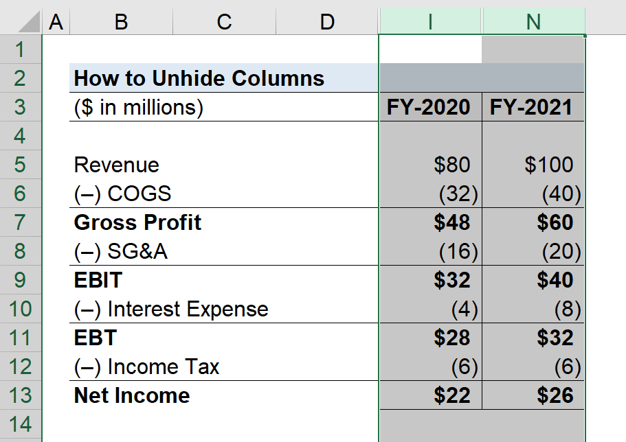
For example, let’s say that we want to unhide columns “J” to “M”, which are the quarterly financials results for fiscal year 2021.
We’d want to highlight columns “I” to “N”, as the screenshot below shows.
The following four steps can be followed to unhide the quarterly results from fiscal year 2021.
- Step 1: Select Cell in Column I
- Step 2: Press Command + Space Bar
- Step 3: Press the Right Arrow to Highlight the Range (“I” to “N”)
- Step 4: ALT → H → O → U → L
Once the steps above are followed, the historical financials for Q-1 to Q-4 in 2021 should be unhidden, whereas the quarterly results from 2020 remain hidden.


Best tutorial on the internet for unhiding hidden columns ever. Thanks